Dataset
This section aims to present the data involved in this practice session. We rely on freely available data, disposed as the Tokyo dataset. In the following part, we explain how to download and prepare this datasets in order to be ready for the practice session.
Description
The Tokyo dataset consists in one Sentinel-2 image and one rasterized Open Street Map (OSM) vector layer. It will be used for all exercises of this section. This dataset has been used during the tutorial at IGARSS 2019 Japan and in the Deep learning on remote sensing images with open-source software book published in 2020.
Remote sensing imagery
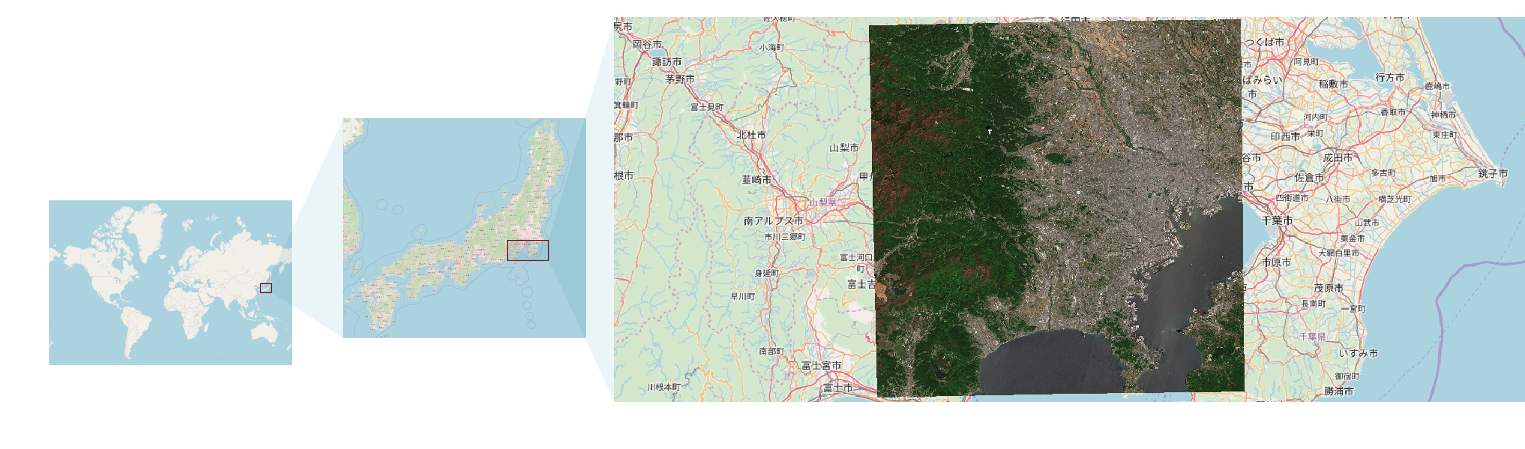
We use a Sentinel-2 image acquired over the Japan mainland, in the area of Tokyo.
We will use the Microsoft Planetary Computer to access the Sentinel-2 product. The following code performs these steps:
- Search the Sentinel-2 image acquired over the Tokyo area at 2019/05/08,
- Get the URLs for the spectral bands geotiffs,
- Process on-the-fly the images to create two local files with the stacked channels respectively for the spectral bands at 10 meters and 20 meters.
from pystac_client import Client
from planetary_computer import sign_inplace
import pyotb

# Search the product
api = Client.open("https://planetarycomputer.microsoft.com/api/stac/v1")
results = api.search(
    bbox=[139.4848, 35.4485, 139.7333, 35.6606],
    datetime="2019-05-08/2019-05-08",
    collections=["sentinel-2-l2a"],
)

# Grab the first result (there should be only one!)
res = next(results.items())

# Create two rasters for the 10m and 20m bands
stacks = {
    "/data/s2_tokyo_10m.tif": ["B02", "B03", "B04", "B08"],
    "/data/s2_tokyo_20m.tif": ["B05", "B06", "B07", "B8A", "B11", "B12"],
}
for filename, bands in stacks.items():
    urls = [sign_inplace(res.assets[key].href) for key in bands]
    concat = pyotb.ConcatenateImages(il=urls)
    concat.write(filename, ext_fname="gdal:co:COMPRESS=DEFLATE", pixel_type="int16")
Run the python script.
Once the product has been processed, you can look into the resulting local files. The product has two sets of images: one is 10m spacing (spectral bands 2, 3, 4 and 8) and the other is 20m spacing (spectral bands 5, 6, 7, 8a, 11 and 12). We won't use the other spectral bands in this section since they are mostly related to atmospheric contents.
| Raster file | Product type | Image size | Pixel encoding | Pixel spacing (meters) |
|---|---|---|---|---|
| /data/s2_tokyo_10m.tif | Multispectral | 10980 x 10980 | int (16 bits) | 10m |
| /data/s2_tokyo_20m.tif | Multispectral | 5490 x 5490 | int (16 bits) | 20m |
Terrain truth
We will use some terrain truth provided by the TETIS research facility of the Montpellier University, France (special thanks to Kenji Osé). The terrain truth is available online, hosted on github. The terrain truth consists in two rasters of labels. Pixels encode classes values, at the same spatial extent and resolution as the 10m image. The corresponding classes are detailed in the table below.
| Class number | Description |
|---|---|
| 0 | Water |
| 1 | Golf course |
| 2 | Park and grassland |
| 3 | Buildings |
| 4 | Forest |
| 5 | Farm |
We use two distinct terrain truth sources for training (A) and validation (B).
Download the data of the terrain truth:
- terrain_truth_epsg32654_A.tif: terrain truth (split A)
- terrain_truth_epsg32654_B.tif: terrain truth (split B)
- legend_style.qml: a style sheet file for QGIS
For validation purposes, the terrain truth (terrain_truth_epsg32654_A.tif and terrain_truth_epsg32654_B.tif) has been split in two datasets such as the objects of A do not overlap objects of B. This way, we have two groups of objects that are distinct. When we perform the sample selection, there is no selected position from A and B that come from the same object.
Sampling
The existing framework of the Orfeo ToolBox offers tools for pixel wise or object oriented classification/regression tasks. On the deep learning side, models like CNNs are trained over patches of images rather than batches of single pixel. Hence otbtf ships new OTB applications to deal with patches.
Patches selection
The first step is the sample selection. It consists in selecting the locations of the center of the samples. For patch-based image classification, there is currently two approaches depending on the type of the terrain truth format, with OTB applications:
-
When terrain truth is vector data: one can use the PolygoncClassStatistics (or the PolygoncClassStatistics, which is faster for large vector data) then SampleSelection applications to select patches centers,
-
When terrain truth is raster data: one can use the LabelImageSampleSelection application.
Since our terrain truth is raster, we use the second approach. You can refer to the OTB CookBook to see how to perform the first approach with OTB.
The following code performs the selection of samples:
import pyotb

# Input terrain truth
tt_a = (
    "https://github.com/remicres/otbtf_tutorials_resources/raw/"
    "master/01_patch_based_classification/tokyo_dataset/terrain_truth/"
    "terrain_truth_epsg32654_A.tif"
)
tt_b = (
    "https://github.com/remicres/otbtf_tutorials_resources/raw/"
    "master/01_patch_based_classification/tokyo_dataset/terrain_truth/"
    "terrain_truth_epsg32654_B.tif"
)

# Output samples locations
pos_a = "/data/pos_a.geojson"
pos_b = "/data/pos_b.geojson"

for inref, outvec in zip([tt_a, tt_b], [pos_a, pos_b]):
    pyotb.LabelImageSampleSelection(
        inref=inref,
        nodata=255,
        outvec=outvec,
        strategy="constant",
        strategy_constant_nb=100,
    )
Note that we read the input raster files directly from the github URL, but we could have used the local files as well.
Here:
inrefis the input label image of the terrain truth,outvecis the output vector data of points for the physical position of samples,strategyis the sampling strategy: "constant" mode enables the sampling of an identical amount of samples in each class. This amount is set using thestrategy_constant_nbparameter,
Run the code.
Question
Once samples positions are computed, open QGIS and import the new vector layers to check that everything has been done correctly.
Patches extraction
Now we should have two new vector layers generated at the previous step, for the locations of the centers of the patches:
- /data/pos_a.geojson
- /data/pos_b.geojson
It is time to use the PatchesExtraction application. The following operation consists in extracting patches in the input image, at each location of the /data/pos_a.geojson. In order to train a small CNN later, we will create a set of patches of dimension 16x16 associated to the corresponding label given from the class field of the vector data.
import pyotb

# Input image (10m bands)
img_10m = "/data/s2_tokyo_10m.tif"

# Input samples locations
pos_a = "/data/pos_a.geojson"
pos_b = "/data/pos_b.geojson"

# Output patches files prefixes
prefix_a = "/data/a_"
prefix_b = "/data/b_"

for vec, prefix in zip([pos_a, pos_b], [prefix_a, prefix_b]):
    pyotb.PatchesExtraction(
        source1_il=img_10m,
        source1_patchsizex=16,
        source1_patchsizey=16,
        source1_out=prefix + "img_10m.tif",
        source1_nodata=0,
        vec=vec,
        field="class",
        outlabels=prefix + "labels.tif",
    )
Here:
source1_ilis the input image list of the first source,source1_patchsizexis the patch width of the first source,source1_patchsizeyis the patch height of the first source,source1_outis the output patches image of the first source,vecis the input vector data of the points (samples locations),fieldis the attribute that we will use as the label value (i.e. the class),outlabelsis the output image for the labels.
Run the code.
After this step, you should have generated the following output images, that we will call the training dataset:
- /data/a_img_10m.tif
- /data/a_labels.tif
And also the following output images, that we call the validation dataset:
- /data/b_img_10m.tif
- /data/b_labels.tif
Sampled patches are stored in one single big image that stacks all patches in rows. The motivation is that accessing one unique big file is more efficient than working on thousands of separate very small files stored in the file system, or accessing sparsely located patches in large images. All geospatial metadata is lost in the process.
Note
Best performances to read patches on-the-fly on high performance computing systems are achieved with TFRecords. Converting extracted patches into TFRecords can be done easily with the python API of otbtf (see the Advanced use, TFRecords section). TFRecords can be created from otbtf patches images, of single patches n-uplets (i.e. samples) created with your own custom workflow.
Question
Check the extracted patches in QGIS: - Open the patches as raster, - If needed, chose the same coordinates reference system as the current project (indicated on the bottom right of the window) so that patches can be displayed.