Inference with CNN

Patch-based inference¶

In the part 1, we have trained successfully our CNN model. Now we will apply the model over the Sentinel-2 image (only 10m spacing bands for now) to produce a land cover map. The optimizer is not used anymore, we just employ the model with its fixed weights as updated after the training. This part is called the inference. To perform the inference, we use the TensorflowModelServe application. We know that our CNN input has a receptive field of 16x16pixels and the input name for the S2 image is input. The output of the model is the estimated class, that is the tensor resulting of the Argmax operator, named estimated_labels. We don't use the optimizer node anymore, as it is part of the training procedure: we use only the model subset that computes estimated_labels from input as shown in the figure below.

flowchart TD

i((input)) --> normalization -- 16x16x4 --> c1[conv 5x5 + ReLU]
c1 -- 12x12x16 --> p1[Max Pooling 2x2] -- 6x6x16 --> c2[conv 3x3 + ReLU]
c2 -- 4x4x32 --> p2[Max Pooling 2x2] -- 2x2x32 --> c3[conv 2x2 + ReLU]
c3 -- 1x1x64 --> c4[conv 1x1 + Softmax]
c4 -- 1x1x6 --> argmax -- 1x1x1 --> p((labels))

First, we need to convert our .keras model file into TensorFlow's SavedModel using this python script:

import argparse
import keras

# unused, but required to load the SavedModel since it implements custom
# operators.
import otbtf
from mymetrics import FScore

parser = argparse.ArgumentParser(
    description="Convert a .keras model into TensorFlow SavedModel"
)
parser.add_argument("--model", required=True, help="input keras model file")
parser.add_argument("--savedmodel", required=True, help="output tensorflow savedmodel")
params = parser.parse_args()

model = keras.saving.load_model(params.model)
model.export(params.savedmodel)

We run it using the following command line:

python part_2_savedmodel.py --model /data/models/model1.keras --savedmodel /data/models/model1_savedmodel

As we don't have GPU support for now, it could be slow to process the whole image. We won't produce the map over the entire image (even if that's possible thanks to the streaming mechanism of OTB) but just over a small subset. We do this using the extended filename of the output image, setting a subset starting at pixel $4000, 4000$ with size 1000x1000. This extended filename consists in adding ?&box=4000:4000:1000:1000 to the output image filename. Note that you can also generate a small image subset with the ExtractROI application of OTB, then use it as input of TensorflowModelServe.

import pyotb
import argparse

parser = argparse.ArgumentParser(description="Apply the savedmodel")
parser.add_argument("--savedmodel", required=True, help="savedmodel directory")
params = parser.parse_args()

# Create the application
infer = pyotb.TensorflowModelServe(
    source1_il="/data/s2_tokyo_10m.tif",  # input image
    source1_rfieldx=16,  # receptive field size
    source1_rfieldy=16,
    source1_placeholder="input",  # model input name
    model_dir=params.savedmodel,  # model directory (savedmodel)
    output_names="estimated_labels",  # model output name
)

# Write
infer.write(
    "/data/map1.tif",  # output image filename
    pixel_type="uint8",  # output image encoding
    ext_fname="box=4000:4000:1000:1000",  # subset of the output image
)

Here is a quick explanation of the application parameters:

• source1 is the parameter group for the first image source,
• source1_il is the input image list of the first source,
• source1_rfieldx is the receptive field width of the first source,
• source1_rfieldy is the receptive field height of the first source,
• source1_placeholder is placeholder name corresponding to the the first source in the TensorFlow model,
• model_dir is the directory of the SavedModel,
• output_names is the list of the output tensors that will be produced then generated as output image,
• out is the filename for the output image generated from the TensorFlow model applied to the entire input image.

You can run the script in command line:

python part_2_inference.py --savedmodel /data/models/model1_savedmodel

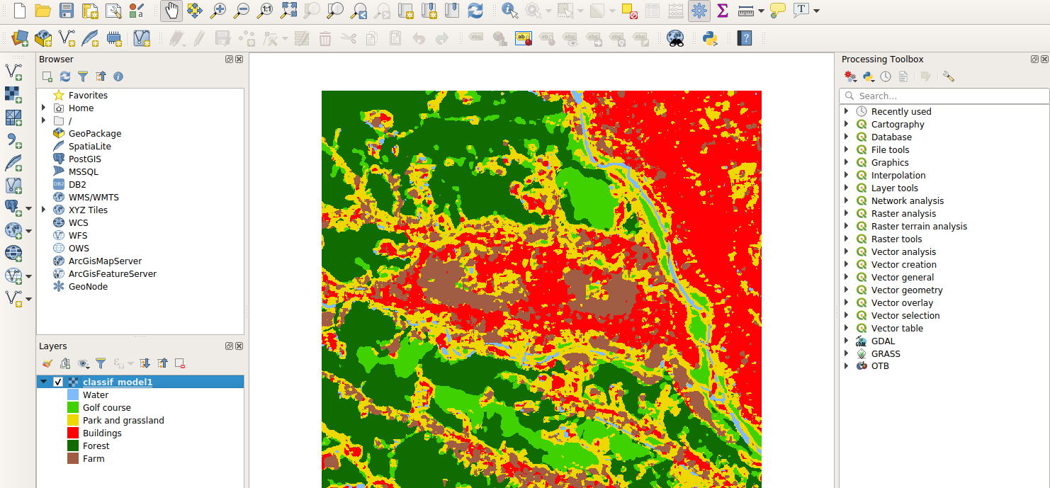
Now import the generated image in QGIS. You can change the style of the raster: in the layers panel (left side of the window), right-click on the image then select Properties, go to the Symbology tab and select render type as single band pseudocolor. Then, you can select the color for each class value, the annotations, etc. You can also load the predefined style by clicking on the Style button (bottom of the window)and opening the file named legend_style.qml that you can download from github.

We just have ran the CNN in patch-based mode, meaning that the application extracts and process patches independently at regular intervals. This is costly, because the sampling strategy requires to duplicate a lot of overlapping patches, and process them independently.

flowchart LR

f([Remote Geotiff files]) -- HTTP --> c[ConcatenateImages]
c --> TensorflowModelServe --> l([Geotiff file])

import pyotb
import argparse
from pystac_client import Client
from planetary_computer import sign_inplace

parser = argparse.ArgumentParser(description="Apply the model")
parser.add_argument("--savedmodel", required=True, help="savedmodel directory")
params = parser.parse_args()

# Retrieve images urls using the STAC API
api = Client.open("https://planetarycomputer.microsoft.com/api/stac/v1")
item_id = "S2A_MSIL2A_20190508T012701_R074_T54SUE_20201006T112414"
item = api.get_collection("sentinel-2-l2a").get_item(item_id)
bands = ["B02", "B03", "B04", "B08"]
urls = [sign_inplace(item.assets[key].href) for key in bands]

# Concatenate
concat = pyotb.ConcatenateImages(il=urls)

# Inference
infer = pyotb.TensorflowModelServe(
    source1_il=concat,
    source1_rfieldx=16,
    source1_rfieldy=16,
    source1_placeholder="input",
    model_dir=params.savedmodel,
    output_names="estimated_labels",
)

# Write
infer.write("/data/map1.tif", pixel_type="uint8", ext_fname="box=4000:4000:1000:1000")

Fully convolutional inference¶

In the previous section, we performed pixel wise classification using a deep convolutional neural network. We have performed the inference in patch-based mode, meaning that for each output pixel, we have run the model on one small patch of the input image, centered on the output pixel position. While this kind of network architecture is easy to implement, it is not efficient in term of processing. Due to patches overlap, the data is copied multiple times with different memory alignment (for each different patch) and passed to the model. The most costly operations implemented in the deep net are the convolutions, which are massively parallel and can be implemented such as the intermediary results are reused for other patches processing (e.g. intermediate sums). However, the patch-based mode disables the possible reuse of the intermediate results since they are re-computed at each new patch, which is not efficient. We will introduce the Fully Convolutional Neural Networks (FCNN, or FCN) that are just CNN that can process entire images regions instead of being limited to small patches.

From the constitution of the simple CNN we used in section, we can notice that this model can be used as a FCN. Its properties are summarized as the following:

• receptive field (16x16 pixels are used at input),
• expression field (1x1 pixel is produced at output),
• scale factor (There is a total of 2 successive pooling operators of size 2, meaning that the scale factor is 4)

We can check that they are consistent with operators implemented in the model: let n be the size of the input image, we can see how will the model propagates the image region to the output of size m:

1. Convolution with 5x5 kernel: output size is $$n-4$$
2. Max pooling with stride (2, 2): output size is $$(n-4)/2=n/2-2$$
3. Convolution with *3x3$ kernel: output size is $$(n/2-2)-2=n/2-4$$
4. Max pooling with stride (2, 2): output size is $$(n/2-4)/2=n/4-2$$
5. Convolution with 2x2 kernel: output size is $$(n/4-2)-1=n/4-3$$

In conclusion, we have $$m=n/4-3$$ which is consistent with the properties (receptive field, expression field, spacing factor) of the model: the model produces an output of size 1x1 from an input image of size 16x16. The physical spacing of its output pixel is equal to the input pixel spacing divided by 4. Run the CNN model with the parameter model_fullyconv to True in order to enable the fully-convolutional processing.

import pyotb
import argparse

parser = argparse.ArgumentParser(description="Apply the model")
parser.add_argument("--savedmodel", required=True, help="savedmodel directory")
params = parser.parse_args()


infer = pyotb.TensorflowModelServe(
    source1_il="/data/s2_tokyo_10m.tif",
    source1_rfieldx=16,
    source1_rfieldy=16,
    source1_placeholder="input",
    model_dir=params.savedmodel,
    output_names="estimated_labels",
    model_fullyconv=True,
)

infer.write(
    "/data/map1_fcn.tif", pixel_type="uint8", ext_fname="box=4000:4000:1000:1000"
)

We can run the inference in command line:

python part_2_inference_fcn.py --savedmodel /data/models/model1_savedmodel

The command should run really quick. You can even run the processing of the entire image.

Open the resulting image in QGIS, and compare with the classification map created by the original CNN. Open the Properties > Metadata tab and check that the physical spacing of the new map is 4 times greater than the original.