Dataset

This section aims to present the data involved for the incoming practice session. We rely on freely available data, disposed as the Paris dataset. The dataset consists in one very high resolution Spot-7 image acquired over the city of Paris, and a label image containing the buildings footprints, water and forest. Note that you can generalize this exercise to any orthorectified remote sensing image at your disposal, and create some terrain truth data by resterizing Open Street Map data over your images.

Geospatial data¶

Spot-7 product¶

The Spot-7 product has been acquired over the city of Paris, France, during summer 2022. It is composed of one multispectral image (6.0 meters physical spacing, Bands: red, green, blue, near infra-red), named xs, and one panchromatic channel (1.5 meters physical spacing, spectral content in visible domain), named pan. This Spot-7 product has been provided by
Dinamis, and its license is open-data (read the terms of conditions here).

You can download the xs and pan files here:

pan
xs

Both rasters are encoded in integer 16 bits, compressed using the deflate algorithm, and stored in GeoTiff format. The coordinate reference system is EPSG:2154 (Lambert 93). Images characteristics are reported in the following table.

Mode	Size	Bands	Physical spacing	Filename
pan	7057x6285	1	1.5 meters	pan.tif
xs	1764x1571	4	6.0 meters	xs.tif

Import the Spot-7 image in QGIS from the menu: Layer > Add layer > Add raster layer then select either the panchromatic channel or the multispectral image of the Spot-7 product.

Labels image¶

As stated before, the terrain truth data has been created over the spot-7 image. It has been created from the French Institute of Geography BD TOPO© at the UMR TETIS Lab. It consist in one raster of single-channel pixels of integers carrying classes labels. The label image has been generated in rasterizing BD TOPO© vector data over the panchromatic channel of the Spot-7 product. Hence its pixels are completely superimposed with the ones of the Spot-7 panchromatic image.

You can download the label image here

The following table summarizes the different classes.

Pixel value	Class description
0	Background
1	Buildings footprints
2	Water surfaces
3	Trees

Sample selection¶

In the following, we will select the center of the patches that we will extract in the images, and that will be used as the terrain truth. We can achieve this step using various tools, and in the following we will address two methods:

QGIS
OTBTF PatchesSelection application

Our goal is to create 3 exclusive groups of point geometries, representing the patches centers for:

the training dataset (80% of patches)
the validation dataset (10% of patches)
the test dataset (10% of patches)

Patches positions seeding in QGIS¶

We can draw vector data in QGIS with the patches centers:

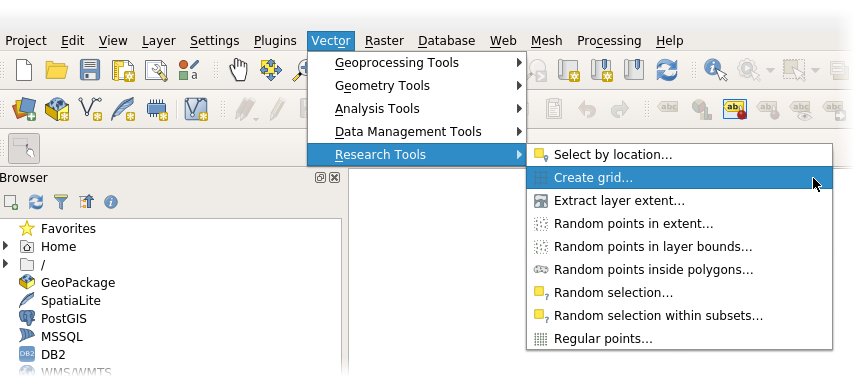
Create a vector grid. Select from the QGIS menu Vector > Research tools > Create grid as shown in the following figure
Create a grid with the following properties:
- Grid type: Rectangle
- Horizontal spacing and Vertical spacing: 96 meters
- Grid extent: select Use extent from then use the Spot-7 image layer to specify the extent.
Now convert this grid of rectangles into centroids using QGIS menu, Vector > Geometry tools > Centroids
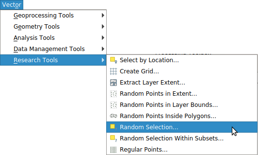
Once the centroids art created, click on the QGIS menu Vector > Research tools > Random Selection
Select this new layer as the input layer, and chose 80 percent of the points to select. Click on execute. Now QGIS should have selected 80 percent of the points.
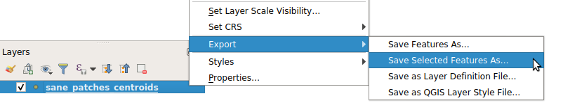
From the layer tab, right-click on the grid layer > export and save the selected features as vec_train.geojson.
Click on the QGIS menu Edit > Selection > Invert selected items
Repeat step 6 with the current selection (which should be the complementary 20 percent of the points) and chose a new file name for the points, e.g. vec_remaining.geojson
Select 50 percent of the points from the vec_remaining.geojson layer, like explained in steps 4 and 5, but applied to the vec_remaining.geojson layer. Export the result like explained in step 6 to vec_valid.geojson. Invert the selection like explained in step 7 and export the other half as vec_test.geojson.

Patches position seeding using OTBTF¶

Another approach is to use the PatchesSelection application of OTB.

part_3_patches_selection.py

import pyotb

pyotb.PatchesSelection(
    {
        "in": "/data/tt.tif",
        "grid.step": 128,  # patch step, in pixels
        "grid.psize": 64,  # patch size, in pixels
        "strategy": "split",
        "strategy.split.trainprop": 0.80,  # proportions
        "strategy.split.validprop": 0.10,
        "strategy.split.testprop": 0.10,
        "outtrain": "/data/vec_train.geojson",  # output files
        "outvalid": "/data/vec_valid.geojson",
        "outtest": "/data/vec_test.geojson",
    }
)

Question

Create part_3_patches_selection.py and run the script,
Open the generated vector data in QGIS, and analyse the spatial layout of the patches centers.

Patches extraction¶

Let's prepare the patches that will be used for training and validation. We use the PatchesExtraction application to extract jointly patches in the Spot-7 images and the label image. In the patch-based part of this tutorial, each remote sensing image patch was associated to a corresponding label value. This time, our goal is slightly different because we need labels as patches, not as a single value like for the patch based approach. Hence, we tell PatchesExtraction that we want three sources: one for the Spot-7 panchromatic image, one for the multispectral image, and one for the label image. We change the OTB_TF_NSOURCES environment variable to 3 to fulfill this need. We extract the patches in positions that we have selected in the previous section, over the following images.

part_3_patches_extraction.py

import pyotb

vec_train = "/data/vec_train.geojson"
vec_valid = "/data/vec_valid.geojson"
vec_test = "/data/vec_test.geojson"

for vec in [vec_train, vec_valid, vec_test]:
    app_extract = pyotb.PatchesExtraction(
        n_sources=3,  # Tells the OTB application to use three sources
        source1_il="/data/pan.tif",
        source1_patchsizex=64,
        source1_patchsizey=64,
        source1_nodata=0,
        source2_il="/data/xs.tif",
        source2_patchsizex=16,
        source2_patchsizey=16,
        source2_nodata=0,
        source3_il="/data/tt.tif",
        source3_patchsizex=64,
        source3_patchsizey=64,
        vec=vec,
        field="id",
    )

    # Create an output filename for pan, xs and labels
    name = vec.replace("vec_", "").replace(".geojson", "")
    out_dict = {
        "source1.out": name + "_p_patches.tif",
        "source2.out": name + "_xs_patches.tif",
        "source3.out": name + "_labels_patches.tif",
    }
    pixel_type = {
        "source1.out": "int16",
        "source2.out": "int16",
        "source3.out": "uint8",
    }
    ext_fname = "gdal:co:COMPRESS=DEFLATE"
    app_extract.write(out_dict, pixel_type=pixel_type, ext_fname=ext_fname)

Question

Create part_3_patches_extraction.py and run the script
Open your patches images in QGIS and check them visually.

The training and validation data are now ready !